Large data, feature hashing and online learning

Note on memory consuption

And at this point it worth to think about how to solve such problem – model matrix with 1/50 of the dataset consumes ~ 200mb. Interpolating to full dataset – matrix will consume ~ 10gb. And this is already a problem for laptop with 16gb RAM. More interestingly it worth to point that at this moment model doesn’t contain any interactions between categorial variables, so prediction power is very limited! Moreover keep in mind that we have 100gb file of views… It becomes obvious that it will be hard to use batch algorithms which requires to kepp all data in RAM.

Note on algorithms and libraries

From my experience linear models work best on such wide high-dimensional sparse data sets. So xgboost (with tree booster) or RanomForest won’t work well. For such tasks I usually use glmnet package, it is also not ideal. For example on my laptop it can fit logistic regression with L1 penalty on matrix above (1/50 of data) for ~ 30 sec. But it consumes ~ 5gb(!) of RAM. Also not that here we check only 10 values of regularization parameter lambda (100 by default).

glmnet_model = glmnet::glmnet(x = X_train, y = y_train, family = 'binomial', 
                      thresh = 1e-3, nlambda = 10, type.logistic = "modified.Newton")

Other interesting packages I’m aware of: pirls, oem, bigLasso (does not support sparse matrices yet). But all of them are not well suited for us due to the size of the problem.

Online learning

It turns out that such large scale high dimensional problems can be efficiently solved in a streaming fashion with stochastic gradient descent. One notable example – vowpal wabbit.

Good thing about SGD is that it requires (O(1)) memory, but also vanilla SGD convergence rate heavily depends on learning rate. Fortunately it was well studied during recent years – it is used as optimization technique in all deep learning applications, used at internet scale ad prediction and so on.

It turns out that using different learning rates for each feature (adaptive learning rates) accelerate convergence drastically. Initial method was AdaGrad by Duchi et al. We will stick to article by McMahan which introduce state-of-the-art FTRL-Proximal algorithm for solving logistic regression with elastic-net penalty. It is proven to be useful in industry and recent CTR kaggle competitions.

FTRL proximal

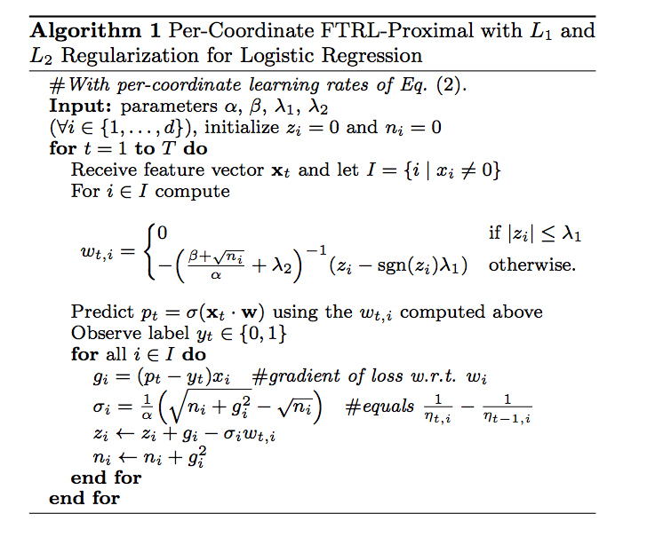
FTRLProximal

I won’t go into details about algorithm, reader can find details in papers above. I will focus on applying it to our problem. Honestrly speaking when I realized necessity of online algorithm, I started to search github for FTRL implementation. And for my surprise I found 3 implementations in R/C/Rcpp – 2 packages – rFTRLProximal, FTRLProximal and pure R implementation in FeatureHashing package (by the way this package allows to create hashed model matrices from data frames – all the stuff we did above manually).

First I tried packages and both of them had some issues:

1. rFTRLProximal didn’t containt possibility of incremental learning
2. FTRLProximal was surprisingly very slow on my sparse data

Then I tried pure R solution from FeatureHashing which was also quite slow (which was not surprise. But it was faster than FTRLProximal!) After some profiling and refactoring I ended with quite fast pure R solution – you can find it on my gist.

And of course during competitions I made a lot of experiments, so didn’t want to wait long minutes while algorithm will converge. So I rewrote it using Rcpp and OpenMP, added dropout regularization and I’m happy to present FTRL package. Let me show it in action:

# first need to isntall it
devtools::install_github("dselivanov/FTRL")

library(Matrix)
library(methods)

library(FTRL)
# First of all need to convert matrix to row-sparse matrix
X_train_csr = as(X_train, "RsparseMatrix")
X_cv_csr = as(X_cv, "RsparseMatrix")
# set up model
ftrl = FTRL$new(alpha = 0.01, beta = 0.1, lambda = 20, l1_ratio = 1, dropout = 0)

As can be noticed FTRL expose partial_fit() method (I follow scikit-learn convention in API). So model can be updated with new data. Or we can fit several epochs on same mini-batch. Let’s check timings with different number of threads:

# 1 thread
system.time(ftrl$partial_fit(X = X_train_csr, y = y_train, nthread = 1))
# 4 threads
system.time(ftrl$partial_fit(X = X_train_csr, y = y_train, nthread = 4))
# 4 threads + 4 hyperthreads
system.time(ftrl$partial_fit(X = X_train_csr, y = y_train, nthread = 8))

Baseline

So now we are done with fast algorithm which can work on laptop. Let’s set up first baseline and put all together:

h_space_size = 2**24
feature_names = c("ad_id", "promo_document_id", "campaign_id", "advertiser_id", "document_id", 
             "platform", "geo_location", "country", "state", "dma")
X_cv = as(X_cv, "RsparseMatrix")
# regularization parameter lambda and learning rate alpha are important hyperparameters
# should be defined after via cross-validation and grid-search
ftrl = FTRL$new(alpha = 0.05, beta = 0.5, lambda = 1, l1_ratio = 1, dropout = 0)
# iterate through all examples 
i = 1
for(i in 0:(N_PART - 1)) {
  dt = events[uuid %% N_PART == i & cv == FALSE]
  dt = clicks_train[dt, on = .(display_id = display_id)]
  dt = promo[dt, on = .(ad_id = ad_id)]
  # create model matrix for a given chunk and convert it to CSR format
  X_train = create_feature_matrix(dt, feature_names, h_space_size) %>% 
    as("RsparseMatrix")
  y_train = as.numeric(dt[, clicked])
  # update model
  ftrl$partial_fit(X = X_train, y = y_train, nthread = 8)
  # check target metric. Alternatively can check map@12
  # but in our case it was 100% correlated with AUC
  if(i %% 5 == 0) {
    train_auc = glmnet::auc(y_train, ftrl$predict(X_train))
    p = ftrl$predict(X_cv)
    dt_cv = data_sample_cv[, .(display_id, clicked, p = -p)]
    # res[, p := -(p)]
    setkey(dt_cv, display_id, p)
    mean_map12 = dt_cv[ , .(map_12 = 1 / .Internal(which(clicked == 1))), by = display_id][['map_12']] %>% 
      mean %>% round(5)
    cv_auc = glmnet::auc(y_cv, p)
    message(sprintf("batch %d train_auc = %f, cv_auc = %f, map@12 = %f",i, train_auc, cv_auc, mean_map12))
  }
}

batch 0 train_auc = 0.724088, cv_auc = 0.705939, map@12 = 0.633280
batch 5 train_auc = 0.731734, cv_auc = 0.717310, map@12 = 0.640460
batch 10 train_auc = 0.733199, cv_auc = 0.720263, map@12 = 0.642470
batch 15 train_auc = 0.734564, cv_auc = 0.721715, map@12 = 0.642940
batch 20 train_auc = 0.735819, cv_auc = 0.722822, map@12 = 0.643520
batch 25 train_auc = 0.736287, cv_auc = 0.723580, map@12 = 0.643700
batch 30 train_auc = 0.735885, cv_auc = 0.723975, map@12 = 0.643940
batch 35 train_auc = 0.736175, cv_auc = 0.724659, map@12 = 0.644270
batch 40 train_auc = 0.737990, cv_auc = 0.725010, map@12 = 0.644170
batch 45 train_auc = 0.737410, cv_auc = 0.725422, map@12 = 0.645230

Along with leak it can bring us to ~150 position on leaderboard.

Baseline 2

One useful thing is to save chunks to disk for further model tuning, so will save model matrix for each mini-batch with wrapper of saveRDS function:

# by default saveRDS can save file with compression level = 6 - very slow
# or without compression - large files.
save_rds_compressed = function(x, file, compr_lvl = 1) {
  con = gzfile(file, open = "wb", compression = compr_lvl)
  saveRDS(x, file = con)
  close.connection(con)
}

Obvious thing to try is to add feature intercations and check how it will improve our model. In order to add interaction we need to modify our create_feature_matrix function. Interactions can be modelled as sum of corresponding underlying features because same combinations of features will be projected into the same values.

# now features will be a list of sets of features
# single values will correspont to single original features, 
# while sets of features will correspond to interactions
# for example `features = list("platform", c("country", "campaign_id") )`
create_feature_matrix = function(dt, features,  h_space_size) {
  # 0-based indices
  row_index = rep(0L:(nrow(dt) - 1L), length(features))
  # note that here we adding `text2vec:::hasher(feature, h_space_size)` - hash offset for this feature
  # this reduces number of collisons because. If we won't apply such scheme - identical values of 
  # different features will be hashed to same value
  col_index = Map(function(fnames) {
    # here we calculate offset for each feature
    # hash name of feature to reduce number of collisions 
    # because for eample if we won't hash value of platform=1 will be hashed to the same as advertiser_id=1
    offset = text2vec:::hasher(paste(fnames, collapse = "_"), h_space_size)
    # calculate index = offest + sum(feature values)
    index = (offset + Reduce(`+`, dt[, fnames, with = FALSE])) %% h_space_size
     as.integer(index)
   }, features) %>% 
    unlist(recursive = FALSE, use.names = FALSE)
  m = sparseMatrix(i = row_index, j = col_index, x = 1,
                   dims = c(nrow(dt), h_space_size),
                   index1 = FALSE, giveCsparse = FALSE, check = F)
  m
}

And know we can create model matrix with some interactions:

interactions = c('promo_document_id', 'campaign_id', 'advertiser_id', 'document_id', 'platform', 'country', 'state') %>% 
  combn(2, simplify = F)
single_features = c('ad_id', 'campaign_id', 'advertiser_id', 'document_id', 'platform', 'geo_location', 'country', 'state', 'dma')
features_with_interactions = c(single_features, interactions)
h_space_size = 2**24
data_sample_cv = data_sample[cv == TRUE]
X_cv = create_feature_matrix(data_sample[cv == TRUE], features_with_interactions, h_space_size) %>% 
  as("RsparseMatrix")
y_cv = as.numeric(data_sample[cv == TRUE, clicked])
save_rds_compressed(list(x = X_cv, y = y_cv, 
                 dt = data_sample_cv[, .(display_id, uuid, ad_id, promo_document_id, campaign_id, advertiser_id)]), 
            file = "~/projects/kaggle/outbrain/data/dt_cv_0.rds")

As we will see process of each batch will take ~ 15 seconds. However on subsequent runs it will be much faster, because we will read model matrix for each minibatch from disk.

# will save mini-batches here
events_matrix_dir = "~/projects/kaggle/outbrain/data/events_matrix/"
dir.create(events_matrix_dir)
# iterate through all examples 
for(i in 0:(N_PART - 1)) {
  dt = events[uuid %% N_PART == 0 & cv == FALSE]
  dt = clicks_train[dt, on = .(display_id = display_id)]
  dt = promo[dt, on = .(ad_id = ad_id)]
  setkey(dt, display_id, ad_id)
  # create model matrix for a given chunk and convert it to CSR format
  X_train = create_feature_matrix(dt, features_with_interactions, h_space_size) %>% 
    as("RsparseMatrix")
  y_train = as.numeric(dt[, clicked])
  # save file for further faster model tuning - we won't need to recalculate model matrix each time
  # dt will be used in further steps to join with page views.
  save_rds_compressed(list(x = X_train, y = y_train, 
                 dt = dt[, .(uuid, ad_id, promo_document_id, campaign_id, advertiser_id)]), 
            file = sprintf("%s/%d.rds", events_matrix_dir, i))
  message(sprintf("%s batch %d", Sys.time(), i))
}

2017-02-04 18:55:58 batch 0
2017-02-04 18:58:46 batch 10
2017-02-04 19:01:29 batch 20
2017-02-04 19:04:14 batch 30
2017-02-04 19:06:56 batch 40

# regularization parameter lambda and learning rate alpha are important hyperparameters
# should be defined after via cross-validation and grid-search
ftrl = FTRL$new(alpha = 0.05, beta = 0.5, lambda = 1, l1_ratio = 1, dropout = 0)
for(i in 0:(N_PART - 1)) {
  data = readRDS(sprintf("%s/%d.rds", events_matrix_dir, i))
  # update model
  ftrl$partial_fit(X = data$x, y = data$y, nthread = 8)
  # check target metric. Alternatively can check map@12
  # but in our case it was 100% correlated with AUC
  if(i %% 5 == 0) {
    train_auc = glmnet::auc(y_train, ftrl$predict(X_train))
    p = ftrl$predict(X_cv)
    dt_cv = data_sample_cv[, .(display_id, clicked, p = -p)]
    setkey(dt_cv, display_id, p)
    mean_map12 = dt_cv[ , .(map_12 = 1 / .Internal(which(clicked == 1))), by = display_id][['map_12']] %>% 
      mean %>% round(5)
    cv_auc = glmnet::auc(y_cv, p)
    message(sprintf("%s batch %d train_auc = %f, cv_auc = %f, map@12 = %f", Sys.time(), i, train_auc, cv_auc, mean_map12))
  }
}

2017-02-04 19:23:41 batch 0 train_auc = 0.720479, cv_auc = 0.710925, map@12 = 0.635120
2017-02-04 19:23:58 batch 5 train_auc = 0.736508, cv_auc = 0.725156, map@12 = 0.645800
2017-02-04 19:24:13 batch 10 train_auc = 0.740824, cv_auc = 0.729285, map@12 = 0.648530
2017-02-04 19:24:28 batch 15 train_auc = 0.743680, cv_auc = 0.731567, map@12 = 0.650900
2017-02-04 19:24:44 batch 20 train_auc = 0.745372, cv_auc = 0.733235, map@12 = 0.651650
2017-02-04 19:25:00 batch 25 train_auc = 0.746855, cv_auc = 0.734358, map@12 = 0.652510
2017-02-04 19:25:15 batch 30 train_auc = 0.748017, cv_auc = 0.734902, map@12 = 0.652590
2017-02-04 19:25:31 batch 35 train_auc = 0.748976, cv_auc = 0.736185, map@12 = 0.653550
2017-02-04 19:25:48 batch 40 train_auc = 0.749709, cv_auc = 0.736798, map@12 = 0.653320
2017-02-04 19:26:03 batch 45 train_auc = 0.750500, cv_auc = 0.737207, map@12 = 0.654440

Again, with leak (which add ~ 0.015) this will give score ~ 0.67 bring to ~ 90-100 position on leadderboard. Please, note time we spend for data preparation and model fitting – we were able to get into top 100 in 20-25 minutes on a laptop.